3Part II: Discovering/Mitigating Bias in Machine Learning
In applications of machine learning as a predictive modeling tool, our model may be biased against some sensitive group. As such, it becomes imperative to find methods of uncovering and reducing any such biases.
3.1 Comparison to Part I
First, recall our notation:
As before with C, think of X as, at first, consisting of all variables other than Y and S, but then selecting some of X as O, with X then being all variables except Y, S and O.
Y: outcome variable, to be predicted
X: variables to be used to predict Y
S: sensitive variable
O: proxy variables
We wish to predict Y from X, either omitting S or reducing its impact, but with concern that we may be indirectly using S via O. But there is a large amount of variation in which fair ML methods actually handle S and O.
Some methods do not deal with O explicitly, merely aiming to “reduce the influence of S,” which implicitly means controlling the impact of O as well.
Some methods aim to eliminate the effect of S entirely, which may implicitly mean eliminating O as well.
Other methods may deal with O explicitly.
Contrast this from our material in Part I:
In Part I, we fit models for predicting Y, but with the goal of using such models to assess the effect of S on Y; we were not interested in actually predicting Y. We included S in our models, but wished to find variables C that were correlated with both Y and S, so as to avoid distorting our look at the impact of S on Y. Any X variable unrelated to Y was not of interest.
Here in Part II, prediction of Y is our central goal, rather than effect assessment. We will either omit S or reduce its impact, possibly in concert with action regarding O.
3.1.1 The Fairness-Utility Tradeoff
The role of the O variables is key. On the one hand, we are worried that they would indirectly allow S to influence predictions – Fairness – but on the other hand, omitting them would reduce our predictive power – Utility. We hope to find a good middle ground.
3.1.2 Exploring proxies
As a preliminary step, the analyst may wish to identify possible proxies. The function dsldOHunting calculates the correlations between S and possible proxies O.
Here’s an example, using the COMPAS data:
library(dsld)data(compas1) # omit decile; we are developing our own # risk recidivism toolcmp <- compas1[,-3] dsldOHunting(cmp,'two_year_recid','race')
The output here shows a trend under which older age suggests that the person is not Black, while a higher prior count indicates the opposite. Neither correlation is large (and they are subject to sampling variation anyway), but together these two variables may cause our predictions to be somewhat biased against African-Americans.
possibly using, say, the age and priors count variables as proxies.
The function does not use the classic Pearson product moment correlation here, opting instead for Kendall’s tau correlation. Both are widely-used, and both take on values in [-1, 1], but while Pearson is geared toward continuous numeric variables, Kendall is also usable for binary or ordinal integer-valued variables.
Tau is defined in terms of concordances and discordances. Say we look at height and weight, and compare two people. If one of the people is both taller and heavier than the other, that is a concordance. If on the other hand, one is shorter but heavier than the other, that is a discordance. We consider all possible pairs of people in our dataset, then set tau to the difference in concordance and discordance counts, divided by the number of pairs.
3.2 Measuring utility
Utility in ML classification algorithms in general, and both utility and fairness in the fair ML classification realm, often (but far from always) make use of quantities like False Positive Rate (FPR). So, let’s start by defining these rates.
NoteThe famous rates FPR etc.
These are conditional probabilities, but it’s important not to confuse the event with the condition.
Consider binary Y classification problems, where we label Y as either positive (e.g. patient has the disease) or negative (e.g. patient does not have the disease).
After we fit our ML tool to predict Y, we use it for prediction. Consider a long period of time in which we do such predictions. During that time, define the following counts:
FP: Count of the number of times we predict Y to be positive and actually it’s negative.
FN: Count of the number of times we predict Y to be negative and actually it’s positive.
TP: Count of the number of times we predict Y to be positive and actually it’s positive.
TN: Count of the number of times we predict Y to be negative and actually it’s negative.
Then some key rates are:
FPR: FP / (FP + TN) = P(guess Y positive | Y actually is negative)
TPR: TP / (TP + FN) = P(guess Y positive | Y actually is positive)
FNR: FN / (TP + FN) = P(guess Y negative | Y actually is positive)
TNR: TN / (FP + TN) = P(guess Y negative | Y actually is negative)
So for instance, FPR is the proportion of time we guess positive, among those times in which Y is actually negative. Two other common terms:
recall: same as TPR
sensitivity: same as TPR
precision: P(Y is actually positive | we guess Y is positive)= TP / (TP + FP)
It is standard to guess Y = 1 if the probability of that event is at least 0.5. But other thresholds can be used, with TPR and FPR varying as we vary the threshold. The ROC curve is the resulting graph of TPR vs. FPR; see qeROC in the qeML package.
A simple but quite common measure of utility in binary classification problems is the overall misclassification probability ; qeML predictive functions report this in the testAcc component of the functions’ return object. There are many, many other measures.
The F1-score has recently been especially popular in the ML research world. It is defined as the harmonic mean of precision and recall, and is thought by some to be especially useful in applications in which one class or the other is very rare.
For whatever reason, ML research has tended to focus on that binary Y case, and there are no analogous acronyms for numeric Y. Accuracy of the latter is handled simply as Mean Squared Prediction Error (MSPE), the average squared difference between predicted and actual Y value, or Mean Absolute Prediction Error (MAPE).
3.3 Measuring unfairness
Many unfairness criteria have been proposed. We present a few of them in this section. It should be kept in mind that, just as there is no single ML algorithm that predicts the best in all applications, one’s choice of fairness measure also will depend on the given application.
See the Xiang and Raji for an excellent analysis of the legal implications of various fairness measures.
3.3.1 S-Correlation
A direct way to measure where Y and S are still related in spite of physically omitting the latter is to compute the correlation between predicted Y, to be denoted Y_{pred} and S. As noted earlier, we use Kendall’s Tau correlation here.
For instance, let’s consider our COMPAS example, say with k-Nearest Neighbors as our ML prediction tool:
Here and below, to keep things simple, we will not use a holdout set.
library(dsld)library(qeML)z <-qeKNN(cmp[, names(cmp) !='race'],'two_year_recid',holdout=NULL,yesYVal='Yes')# look at the fitted model's probability of recidivism,# i.e. regression estimatesprobs <- z$regests# the variable 'race' is an R factor, need a numericblack <-ifelse(cmp$race=='African-American',1,0)cor(black,probs,method='kendall')
[1] 0.1765781
That’s a pretty substantial correlation, definitely a cause for concern that our ML analysis here is unfair. Of course, it’s not the algorithm itself’s fault, but we must find a way to mitigate the problem.
3.3.2 Demographic Parity
The criterion for demographic parity is that the same proportion of each subgroup within the sensitive feature is classified at equal rates for each of the possible outcomes
For example, let’s consider the COMPAS dataset again. Demographic Parity would require
z <-qeKNN(cmp[, names(cmp) !='race'],'two_year_recid',holdout=NULL,yesYVal='Yes')# determine which rows were for Black applicants, which notBlackRows <-which(cmp$race =='African-American')NonblackRows <-setdiff(1:nrow(cmp),BlackRows) # all the others# regests, the output of qeKNN, is the vector of fitted probabilities# (recall that for the Y = 0,1 case, the mean reduces to the probability# of a 1)BlackProbs <- z$regests[BlackRows]NonblackProbs <- z$regests[NonblackRows]# if a probability is > 0.5, we will guess Y = 1, otherwise guess Y = 0BlackYhats <-as.integer(BlackProbs >0.5)NonblackYhats <-as.integer(NonblackProbs >0.5)# again, recall that the mean of a bunch of 0s and 1s is the proportion# of 1s, i.e. the probability of a 1mean(BlackYhats)
[1] 0.5059504
mean(NonblackYhats)
[1] 0.3174331
That’s quite a difference! Overall, our ML model predicts about 51% of Black defendants to recidivate, versus 32% for non-Blacks.
However, such a criterion is generally considered too coarse, since it doesn’t account for possible differences in qualifications between the two groups. In other words, one must take confounders into account, as we did in Part I.
3.3.3 Equalized Odds
This criterion takes a retrospective view, asking in the case of COMPAS:
Among those who recidivate, what proportion of them had been predicted to do so? And, does that proportion vary by race?
If the answer to that second question is No, we say our prediction tool satisfies the Equal Opportunity criterion, which is one part of Equalized Odds.
So, Equalized Odds requires both quantities
TP / (TP+FN) and FP / (FP+TN)
to be the same for each sensitive group.
3.3.4 The fairness package
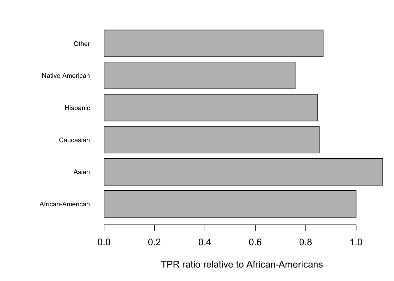
This package calculates and graphically displays a wide variety of fairness criteria. For instance, it can evaluate the Equalized Odds criterion in the above COMPAS example. Despite its name, equal_odds() compares only true positive rates, the Equal Opportunity component of Equalized Odds. The package is now archived on CRAN, so we calculate the same rates directly:
            African-American      Asian    Caucasian    Hispanic
Sensitivity        0.7536694  0.8333333    0.6433824   0.6378378
TPR ratio          1.0000000  1.1057014    0.8536665   0.8463098
Group size      2941.0000000 28.0000000 2055.0000000 501.0000000
            Native American       Other
Sensitivity       0.5714286   0.6551724
TPR ratio         0.7581952   0.8693101
Group size       14.0000000 316.0000000
par(mar=c(5,9,2,1))barplot(tprRatio, horiz=TRUE, las=1, cex.names=0.7,xlab='TPR ratio relative to African-Americans')
Taking African-Americans as the base, we see that the Equalized Odds criterion was not met, even approximately. Nor was Demographic Parity.
3.4 Remedies
Having established that ML prediction models can be biased against certain sensitive groups, what remedies are available? The dsld package includes a few of these, presented in this section. Of course, all of them recognize the basic principle that we stated earlier:
NoteThe Fairness-Utility Tradeoff
Of course, nothing comes for free: the inherent tradeoff of increasing fairness is reduced utility (reduced predictive power over the dataset). Thus, a means of balancing this tradeoff between fairness and utility becomes essential in any future implementations of machine learning.
Any algorithm for ameliorating unfairness will thus include one or more parameters that one can use to achieve a desired level of compromise between fairness and utility. The parameters essentially allow us to “dial” the weight that our proxies will play in predicting Y; lighter weight means more fairness but poorer utility, and vice versa.
Many, many fair ML algorithms have been proposed, most of which are technically complex. The ones we present here have been chosen (a) for their technical simplicity and (b) availability as R packages. We will begin with the simplest algorithms (which have been developed by one of the authors of this book).
Let’s take as a running example the COMPAS data, predicting recidivism, with age and prior convictions count as proxies. To illustrate prediction, we will predict the first case in the dataset:
newx <- cmp[1, names(cmp) !='two_year_recid'] # X and S; omit Y
S is included only for optional correlation diagnostics; EDF predictions use X alone. A single case is not enough to estimate a correlation.
3.5 Functions based on the Explicitly Deweighted Features (EDF) Method
explicitly reducing the weights of the O variables, according to user specification
The deweighting parameters are set via an argument deweightPars in the function calls. This argument takes the form of an R list, with one component for each variable in the user’s O set. The meanings of the parameters will vary according to the ML algorithm used, as seen below.
3.5.1dsldQeFairRF
This function fits an RF model, but with deweighting of the proxies.
African-American            Asian        Caucasian         Hispanic
     0.127712333     -0.027685081     -0.078637154     -0.049746267
 Native American            Other
    -0.003057229     -0.045801064
predict(z,newx)$preds
$predClasses
[1] No
Levels: No Yes

$probs
             0         1
[1,] 0.6325785 0.3674215
The meaning of the deweighting parameters in this function is as follows: Recall that in RFs, each tree will use a different random ordering of the X variables. At any given node in a tree, a variable is chosen at random to set up a possible split point. But here we are specifying that the age and priors count variables be used only 20% and 10% as often as other variables, in order to reduce their impact.
Yet the S-Correlation values are still nonzero, especially in the Black and Caucasian cases. We need to give the O variables even smaller weights or possibly include additional variables in our O set.
3.5.2dsldQeFairKNN
The role of the deweighting parameters in this k-NN implementation of EDF is as follows: We use weighted distances in finding near neighbors. Ordinarily, if we move 3.2 meters to the right and then 1.1 meters forward, the distance between our new point and our original one is
\sqrt{3.2^2+1.1^2} \approx 3.38
That puts equal weight in the left-right direction and the forward-back direction, which makes sense for geometric distance. But in data prediction, we can use different weights. In predicting wage income in the Census data, say, we can place large weight on age and occupation, and less weight on education. Our COMPAS data call would work in this manner:
z <-dsldQeFairKNN(cmp,'two_year_recid','race',list(age=0.2,priors_count=0.1),yesYVal='Yes')knnProbs <- z$trainPreds$preds$probssapply(levels(cmp$race), function(r)cor(cmp$race == r, knnProbs, method='kendall'))
African-American            Asian        Caucasian         Hispanic
     0.140941888     -0.027014389     -0.092626030     -0.045893605
 Native American            Other
     0.001746851     -0.051539781
predict(z,newx)$preds
$predClasses
[1] Yes
Levels: No Yes

$probs
[1] 0.56
3.5.3dsldQeFairRidgeLin and dsldQeFairRidgeLog
One of the most striking advances in modern statistics was the discovery that classical estimators tend to be “too big,” and that one may improve accuracy by “shrinking” them. Here is the intuition:
Consider the example in Section 2.6. The vector of estimated regression coefficients was
(12.46,-0.094,0.39,0.16,…)
We might (crudely) shrink this vector by multiplying by a factor of, say, 0.5, yielding
(6.23,-0.047,0.20,0.08,…)
The actual shrinkage mechanisms used in the regression context are much more complex than simply multiplying every component of the vector by the same constant, but this is the basic principle.
Why might this odd action be helpful? Shrinking introduces a bias, but reduces variance (roughly speaking, smaller variables vary less). If outliers (extreme values, not errors) are common in the data, these result in large estimator variance, possibly so much that shrinkage’s reduction in variance more than compensates for our increase in bias.
Some readers may have heard of ridge regression and the LASSO, both of which impose shrinkage. For our EDF context, though, we wish to perform our shrinkage focusing on only some of the estimated regression coefficients, specifically those corresponding to our proxies. To be sure, it should be noted that non-proxy coefficients are affected too, but the main effects will be on the proxies. This is what dsldQeFairRidgeLin and dsldQeFairRidgeLog do, with linear and logit cases.
Note that these estimators also have the potential ancillary benefit obtained from shrinkage in general, i.e. better utility.
3.6 Wrappers for fairML functions
We consider here dsldFrrm and dsldFgrrm, wrappers to functions in the fairml package, based on a paper by the authors of the package. Their methods apply a ridge penalty to S, thus reducing its influence. Note that contrast to EDF:
The fairML functions aim to address the fairness issue through an argument unfairness, a number in (0,1]. The smaller the value, the fairer the fit.
EDF omits S from its analysis; the fairML functions retain S, and in fact compute regression coefficients for it.
EDF has multiple inputs for deweighting, while fairML has a single parameter.
EDF explicitly deweights the O variables, under the control of the user; fairML does so only indirectly via their relation to S, without user input.
Of course, each may work better than the other for any particular dataset.
Let’s see what it does with the COMPAS data, trying three different values of unfairness:
set.seed(9999)# Display the fitted model, without printing every training prediction.dsldFgrrm(cmp,'two_year_recid','race',unfairness=1.0,family='binomial',yesYVal='Yes')$base
The first value, 1.0, yielded a Caucasian coefficient of -0.73, which then shrank to -0.37 with unfairness = 0.1, and then to -0.03 with unfairness = 0.01. (Note that the base for the dummy variables is apparently African-American.) There seems to be rather little effect on our possible proxies, age and priors count.